Neuronales Netz
Contents
Neuronales Netz
One-Hot-Encoding
import numpy as np
from numpy import load
from scipy.special import expit
from sklearn.preprocessing import OneHotEncoder
import pickle
import matplotlib.pyplot as plt

# load numpy array from npy file

X_train=load('../01_Dataset/dataset_28x28/X_train.npy').astype(np.float32) * 1.0/255.0 # normalisieren
y_train=load('../01_Dataset/dataset_28x28/y_train.npy')
X_test=load('../01_Dataset/dataset_28x28/X_test.npy').astype(np.float32) * 1.0/255.0  # normalisieren
y_test=load('../01_Dataset/dataset_28x28/y_test.npy')

print(X_train.shape)
print(len(y_train))
print(X_test.shape)
print(len(y_test))

# one-hot-encoding
oh = OneHotEncoder()
y_train_oh = oh.fit_transform(y_train.reshape(-1, 1)).toarray()
(6421, 28, 28, 1)
6421
(2753, 28, 28, 1)
2753
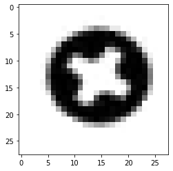
# label check
i=5
print("Label y_train: " + str(y_train[i]))
print("Label y_train (One-Hot-Encoded): " + str(y_train_oh[i]))
plt.imshow(X_train[i],cmap='gray')
plt.show

# Kategorien:
# 0: innensechskant
# 1: philips
# 2: pozidriv
# 3: sechskant
# 4: torx
Label y_train: 1
Label y_train (One-Hot-Encoded): [0. 1. 0. 0. 0.]
<function matplotlib.pyplot.show(close=None, block=None)>
X_train = X_train.astype(np.float32).reshape(-1, 784) # reshape hier wegen label test
X_test  = X_test.astype(np.float32).reshape(-1, 784) #
y_test = y_test.astype(np.int32)

print(X_train)
print(X_test.shape)
print(y_test)
[[1. 1. 1. ... 1. 1. 1.]
 [1. 1. 1. ... 1. 1. 1.]
 [1. 1. 1. ... 1. 1. 1.]
 ...
 [1. 1. 1. ... 1. 1. 1.]
 [1. 1. 1. ... 1. 1. 1.]
 [1. 1. 1. ... 1. 1. 1.]]
(2753, 784)
[3 0 1 ... 1 0 3]
Neuronales Netz
# Quelle: Jannis Seemann , Udemy-Kurs Deep Learning
class NeuralNetwork(object):
    def __init__(self, lr = 0.01):
        self.lr = lr

        self.w0 = np.random.randn(100, 784)
        self.w1 = np.random.randn(5, 100)


    def activation(self, x):
        return expit(x)

    def train(self, X, y):
        a0 = self.activation(self.w0 @ X.T)
        pred = self.activation(self.w1 @ a0)

        e1 = y.T - pred
        e0 = e1.T @ self.w1

        dw1 = e1 * pred * (1 - pred) @ a0.T / len(X)
        dw0 = e0.T * a0 * (1 - a0) @ X / len(X)

        assert dw1.shape == self.w1.shape
        assert dw0.shape == self.w0.shape

        self.w1 = self.w1 + self.lr * dw1
        self.w0 = self.w0 + self.lr * dw0

        # print("Kosten: " + str(self.cost(pred, y)))

    def predict(self, X):
        a0 = self.activation(self.w0 @ X.T)
        pred = self.activation(self.w1 @ a0)
        return pred

    def cost(self, pred, y):
        # SUM((y - pred)^2)
        s = (1 / 2) * (y.T - pred) ** 2
        return np.mean(np.sum(s, axis=0))

model = NeuralNetwork()

for i in range(0, 500):
    for j in range(0, len(X_train), 100):
        model.train(X_train[j:(j + 100), :] / 255., y_train_oh[j:(j + 100), :])

    y_test_pred = model.predict(X_test / 255.)
    y_test_pred = np.argmax(y_test_pred, axis=0)
    print(np.mean(y_test_pred == y_test))
0.20232473665092626
0.20232473665092626
0.20232473665092626
0.20232473665092626
0.20232473665092626
0.20232473665092626
0.20232473665092626
0.20232473665092626
0.20232473665092626
0.20232473665092626
0.20232473665092626
0.20232473665092626
0.20232473665092626
0.20232473665092626
0.20232473665092626
0.20232473665092626
0.20232473665092626
0.20232473665092626
0.20232473665092626
0.20232473665092626
0.20232473665092626
0.20232473665092626
0.20232473665092626
0.20232473665092626
0.20232473665092626
0.20232473665092626
0.20232473665092626
0.20232473665092626
0.20232473665092626
0.20232473665092626
0.20232473665092626
0.20232473665092626
0.20232473665092626
0.20232473665092626
0.20232473665092626
0.20232473665092626
0.2026879767526335
0.1914275335997094
0.17689792953142028
0.17580820922629858
0.17108608790410462
0.17253904831093353
0.17653468942971304
0.17835088993824919
0.1787141300399564
0.1808935706501998
0.18307301126044315
0.1848892117689793
0.185978932074101
0.18815837268434435
0.1888848528877588
0.1910642934980022
0.19179077370141664
0.1925172539048311
0.1936069742099528
0.19433345441336725
0.19433345441336725
0.19614965492190337
0.19723937522702506
0.19723937522702506
0.1976026153287323
0.2001452960406829
0.20050853614239011
0.20196149654921902
0.20196149654921902
0.2026879767526335
0.20341445695604796
0.20450417726116962
0.20523065746458408
0.20632037776970577
0.20777333817653468
0.20849981837994916
0.20886305848165637
0.20958953868507083
0.20995277878677807
0.21067925899019252
0.21285869960043588
0.21322193970214312
0.21394841990555757
0.21540138031238648
0.21540138031238648
0.21576462041409372
0.21721758082092263
0.21830730112604432
0.21903378132945878
0.22048674173628768
0.22121322193970214
0.22121322193970214
0.22157646204140938
0.22266618234653104
0.22484562295677443
0.22484562295677443
0.22484562295677443
0.22520886305848165
0.22629858336360334
0.2270250635670178
0.2284780239738467
0.2284780239738467
0.2295677442789684
0.23029422448238285
0.2310207046857973
0.23138394478750454
0.23174718488921178
0.23174718488921178
0.232110424990919
0.2335633853977479
0.23428986560116236
0.23501634580457684
0.23537958590628405
0.2357428260079913
0.2361060661096985
0.2371957864148202
0.23755902651652744
0.23792226661823465
0.2382855067199419
0.23901198692335635
0.2408281874318925
0.2411914275335997
0.24155466763530695
0.24155466763530695
0.24155466763530695
0.2411914275335997
0.24155466763530695
0.24191790773701416
0.2426443879404286
0.24337086814384307
0.24300762804213585
0.24337086814384307
0.24446058844896476
0.244823828550672
0.244823828550672
0.24518706865237921
0.244823828550672
0.24518706865237921
0.24700326916091536
0.2473665092626226
0.24772974936432982
0.24772974936432982
0.2488194696694515
0.24918270977115872
0.2502724300762804
0.2509989102796949
0.2513621503814021
0.2517253904831093
0.2517253904831093
0.2517253904831093
0.25208863058481656
0.25281511078823105
0.2524518706865238
0.2524518706865238
0.25317835088993823
0.25354159099164547
0.25463131129676714
0.2549945513984744
0.2553577915001816
0.25572103160188886
0.2564475118053033
0.2564475118053033
0.2586269524155467
0.25971667272066834
0.2604431529240828
0.2604431529240828
0.26225935343261897
0.26225935343261897
0.2626225935343262
0.2629858336360334
0.26443879404286236
0.26480203414456954
0.26589175444969126
0.26589175444969126
0.26698147475481293
0.26734471485652017
0.26734471485652017
0.2680711950599346
0.2680711950599346
0.2680711950599346
0.26843443516164184
0.2695241554667635
0.2691609153650563
0.2695241554667635
0.26988739556847074
0.270250635670178
0.270250635670178
0.2706138757718852
0.2717035960770069
0.27206683617871413
0.2727933163821286
0.2731565564838358
0.2738830366872503
0.2731565564838358
0.2738830366872503
0.2746095168906647
0.2753359970940792
0.2753359970940792
0.278241917907737
0.2789683981111515
0.28078459861968763
0.28223755902651654
0.28296403922993096
0.28223755902651654
0.2826007991282238
0.2826007991282238
0.2826007991282238
0.2833272793316382
0.2840537595350527
0.2855067199418816
0.28586996004358883
0.286233200145296
0.286233200145296
0.28732292045041774
0.287686160552125
0.28877588085724665
0.2898656011623683
0.2905920813657828
0.29168180167090446
0.2920450417726117
0.2920450417726117
0.29386124228114785
0.2945877224845623
0.29531420268797676
0.2960406828913912
0.29894660370504905
0.29894660370504905
0.29894660370504905
0.2993098438067563
0.3000363240101707
0.30039956411187796
0.3011260443152924
0.3011260443152924
0.3014892844169996
0.30185252451870687
0.30185252451870687
0.30257900472212135
0.3033054849255358
0.303668725027243
0.303668725027243
0.303668725027243
0.3033054849255358
0.30403196512895025
0.3047584453323647
0.3047584453323647
0.3051216854340719
0.3051216854340719
0.3051216854340719
0.3051216854340719
0.3051216854340719
0.30657464584090083
0.30802760624772973
0.3076643661460225
0.308390846349437
0.3087540864511442
0.30911732655285146
0.30911732655285146
0.30911732655285146
0.31057028695968036
0.31057028695968036
0.3112967671630948
0.31166000726480203
0.31166000726480203
0.31202324736650927
0.3127497275699237
0.31311296767163094
0.3138394478750454
0.3149291681801671
0.3152924082818743
0.3152924082818743
0.316382128586996
0.31674536868870323
0.3174718488921177
0.3185615691972394
0.3192880494006538
0.3192880494006538
0.3200145296040683
0.3200145296040683
0.32037776970577553
0.32074100980748277
0.32110424990918995
0.3221939702143117
0.3229204504177261
0.3229204504177261
0.32328369051943334
0.3236469306211406
0.324373410824555
0.32473665092626225
0.32473665092626225
0.324373410824555
0.324373410824555
0.324373410824555
0.324373410824555
0.324373410824555
0.32473665092626225
0.3250998910279695
0.32582637123138397
0.32691609153650564
0.3272793316382129
0.3280058118416273
0.32836905194333454
0.329095532146749
0.32982201235016345
0.3301852524518707
0.3301852524518707
0.33054849255357793
0.3309117326552851
0.3309117326552851
0.33127497275699236
0.3316382128586996
0.33200145296040684
0.3323646930621141
0.3323646930621141
0.33272793316382127
0.3330911732655285
0.33345441336723575
0.333817653468943
0.3345441336723574
0.33490737377406465
0.3352706138757719
0.3352706138757719
0.33490737377406465
0.33563385397747914
0.3359970940791863
0.33636033418089356
0.3367235742826008
0.33781329458772247
0.3381765346894297
0.33853977479113695
0.3389030148928442
0.3396294950962586
0.3403559752996731
0.3403559752996731
0.3403559752996731
0.3403559752996731
0.34071921540138034
0.34144569560479476
0.34144569560479476
0.34217217580820924
0.34253541590991643
0.34289865601162367
0.34289865601162367
0.34253541590991643
0.34253541590991643
0.34289865601162367
0.34362513621503815
0.3443516164184526
0.3447148565201598
0.3454413367235743
0.34653105702869597
0.34653105702869597
0.34725753723211045
0.3483472575372321
0.3483472575372321
0.3483472575372321
0.34871049763893935
0.3490737377406466
0.3490737377406466
0.3490737377406466
0.3494369778423538
0.3494369778423538
0.3494369778423538
0.3494369778423538
0.349800217944061
0.349800217944061
0.349800217944061
0.3505266981474755
0.3508899382491827
0.3508899382491827
0.3508899382491827
0.35161641845259717
0.35161641845259717
0.3519796585543044
0.3519796585543044
0.3519796585543044
0.3519796585543044
0.35234289865601165
0.35270613875771883
0.3530693788594261
0.35379585906284056
0.35379585906284056
0.35415909916454774
0.35524881946966946
0.35633853977479113
0.3570650199782056
0.3574282600799128
0.3574282600799128
0.35779150018162004
0.35779150018162004
0.35779150018162004
0.3581547402833273
0.3585179803850345
0.3596077006901562
0.3599709407918634
0.36033418089357067
0.36033418089357067
0.36033418089357067
0.36033418089357067
0.36142390119869233
0.3617871413003996
0.362513621503814
0.36287686160552124
0.3632401017072285
0.3636033418089357
0.36396658191064296
0.36396658191064296
0.36432982201235015
0.36578278241917905
0.36650926262259353
0.3668725027243008
0.3668725027243008
0.3668725027243008
0.3668725027243008
0.3668725027243008
0.367235742826008
0.36796222302942244
0.3675989829277152
0.36796222302942244
0.3686887032328369
0.3690519433345441
0.3697784235379586
0.36941518343625135
0.3690519433345441
0.3697784235379586
0.3697784235379586
0.3697784235379586
0.3697784235379586
0.3697784235379586
0.3697784235379586
0.3697784235379586
0.37086814384308026
0.3712313839447875
0.37159462404649474
0.37232110424990916
0.37232110424990916
0.37232110424990916
0.3726843443516164
0.37304758445332364
0.3734108245550309
0.3737740646567381
0.3741373047584453
0.3741373047584453
0.3741373047584453
0.37450054486015255
0.3748637849618598
0.37522702506356703
0.37522702506356703
0.37595350526698146
0.3763167453686887
0.37667998547039594
0.37667998547039594
0.3770432255721032
0.3770432255721032
0.37740646567381037
0.37740646567381037
0.37740646567381037
0.3770432255721032
0.3770432255721032
0.37740646567381037
0.3777697057755176
0.3784961859789321
0.3792226661823465
0.3792226661823465
0.37958590628405375
0.37958590628405375
0.379949146385761
0.379949146385761
0.379949146385761
0.379949146385761
0.38031238648746823
0.3806756265891754
0.38103886669088266
0.3814021067925899
0.3814021067925899
0.3814021067925899
0.3814021067925899
0.38176534689429714
0.38176534689429714
0.38176534689429714
0.38176534689429714
0.38176534689429714
0.38176534689429714
0.3828550671994188
0.3828550671994188
0.3828550671994188
0.3835815474028333
0.3835815474028333
0.3839447875045405
0.3843080276062477
0.3843080276062477
0.38467126770795496
0.3850345078096622
0.38539774791136944
0.38539774791136944
0.3857609880130766
0.3857609880130766
0.3857609880130766
0.3857609880130766
0.3857609880130766
0.38612422811478386
0.3864874682164911
0.3872139484199056
0.3872139484199056
0.3872139484199056
Mehrere Ausgänge
import numpy as np
from tensorflow.keras.utils import to_categorical

from numpy import load
import matplotlib.pyplot as plt

X_train = load('../01_Dataset/dataset_28x28/X_train.npy').astype(np.float32).reshape(-1, 784)*1.0/255.0
y_train = load('../01_Dataset/dataset_28x28/y_train.npy').astype(np.int32)

X_test=load('../01_Dataset/dataset_28x28/X_test.npy').astype(np.float32).reshape(-1, 784)*1.0/255.0
y_test=load('../01_Dataset/dataset_28x28/y_test.npy').astype(np.int32)

y_train = to_categorical(y_train)
y_test = to_categorical(y_test)
from tensorflow.keras.models import Sequential
from tensorflow.keras.layers import Dense

model = Sequential()

model.add(Dense(100, activation="sigmoid", input_shape=(784,)))
model.add(Dense(5, activation="sigmoid"))

model.compile(optimizer="sgd", loss="categorical_crossentropy", metrics=["accuracy"])

model.fit(
    X_train,
    y_train,
    epochs=100,
    batch_size=100)
Epoch 1/100
65/65 [==============================] - 0s 3ms/step - loss: 1.5785 - accuracy: 0.2179
Epoch 2/100
65/65 [==============================] - 0s 3ms/step - loss: 1.4458 - accuracy: 0.5010
Epoch 3/100
65/65 [==============================] - 0s 3ms/step - loss: 1.3253 - accuracy: 0.6337
Epoch 4/100
65/65 [==============================] - 0s 3ms/step - loss: 1.2080 - accuracy: 0.6566
Epoch 5/100
65/65 [==============================] - 0s 3ms/step - loss: 1.1071 - accuracy: 0.6753
Epoch 6/100
65/65 [==============================] - 0s 3ms/step - loss: 1.0270 - accuracy: 0.6887
Epoch 7/100
65/65 [==============================] - 0s 3ms/step - loss: 0.9640 - accuracy: 0.7080
Epoch 8/100
65/65 [==============================] - 0s 3ms/step - loss: 0.9130 - accuracy: 0.7156
Epoch 9/100
65/65 [==============================] - 0s 3ms/step - loss: 0.8719 - accuracy: 0.7273
Epoch 10/100
65/65 [==============================] - 0s 3ms/step - loss: 0.8358 - accuracy: 0.7331
Epoch 11/100
65/65 [==============================] - 0s 3ms/step - loss: 0.8068 - accuracy: 0.7413
Epoch 12/100
65/65 [==============================] - 0s 3ms/step - loss: 0.7801 - accuracy: 0.7475
Epoch 13/100
65/65 [==============================] - 0s 3ms/step - loss: 0.7570 - accuracy: 0.7502
Epoch 14/100
65/65 [==============================] - 0s 3ms/step - loss: 0.7370 - accuracy: 0.7592
Epoch 15/100
65/65 [==============================] - 0s 3ms/step - loss: 0.7185 - accuracy: 0.7653
Epoch 16/100
65/65 [==============================] - 0s 3ms/step - loss: 0.7014 - accuracy: 0.7670
Epoch 17/100
65/65 [==============================] - 0s 3ms/step - loss: 0.6861 - accuracy: 0.7712
Epoch 18/100
65/65 [==============================] - 0s 4ms/step - loss: 0.6715 - accuracy: 0.7784
Epoch 19/100
65/65 [==============================] - 0s 3ms/step - loss: 0.6584 - accuracy: 0.7782
Epoch 20/100
65/65 [==============================] - 0s 3ms/step - loss: 0.6458 - accuracy: 0.7821
Epoch 21/100
65/65 [==============================] - 0s 3ms/step - loss: 0.6347 - accuracy: 0.7835
Epoch 22/100
65/65 [==============================] - 0s 3ms/step - loss: 0.6237 - accuracy: 0.7885
Epoch 23/100
65/65 [==============================] - 0s 3ms/step - loss: 0.6135 - accuracy: 0.7893
Epoch 24/100
65/65 [==============================] - 0s 5ms/step - loss: 0.6035 - accuracy: 0.7893
Epoch 25/100
65/65 [==============================] - 0s 3ms/step - loss: 0.5944 - accuracy: 0.7929
Epoch 26/100
65/65 [==============================] - 0s 3ms/step - loss: 0.5856 - accuracy: 0.7969
Epoch 27/100
65/65 [==============================] - 0s 3ms/step - loss: 0.5771 - accuracy: 0.7974
Epoch 28/100
65/65 [==============================] - 0s 3ms/step - loss: 0.5699 - accuracy: 0.7986
Epoch 29/100
65/65 [==============================] - 0s 2ms/step - loss: 0.5615 - accuracy: 0.8028
Epoch 30/100
65/65 [==============================] - 0s 3ms/step - loss: 0.5546 - accuracy: 0.8008
Epoch 31/100
65/65 [==============================] - 0s 3ms/step - loss: 0.5471 - accuracy: 0.8047
Epoch 32/100
65/65 [==============================] - 0s 3ms/step - loss: 0.5400 - accuracy: 0.8055
Epoch 33/100
65/65 [==============================] - 0s 2ms/step - loss: 0.5340 - accuracy: 0.8081
Epoch 34/100
65/65 [==============================] - 0s 2ms/step - loss: 0.5277 - accuracy: 0.8050
Epoch 35/100
65/65 [==============================] - 0s 3ms/step - loss: 0.5215 - accuracy: 0.8103
Epoch 36/100
65/65 [==============================] - 0s 2ms/step - loss: 0.5155 - accuracy: 0.8123
Epoch 37/100
65/65 [==============================] - 0s 2ms/step - loss: 0.5101 - accuracy: 0.8145
Epoch 38/100
65/65 [==============================] - 0s 3ms/step - loss: 0.5045 - accuracy: 0.8123
Epoch 39/100
65/65 [==============================] - 0s 3ms/step - loss: 0.4994 - accuracy: 0.8162
Epoch 40/100
65/65 [==============================] - 0s 3ms/step - loss: 0.4941 - accuracy: 0.8186
Epoch 41/100
65/65 [==============================] - 0s 3ms/step - loss: 0.4886 - accuracy: 0.8193
Epoch 42/100
65/65 [==============================] - 0s 3ms/step - loss: 0.4846 - accuracy: 0.8193
Epoch 43/100
65/65 [==============================] - 0s 3ms/step - loss: 0.4797 - accuracy: 0.8215
Epoch 44/100
65/65 [==============================] - 0s 3ms/step - loss: 0.4751 - accuracy: 0.8215
Epoch 45/100
65/65 [==============================] - 0s 3ms/step - loss: 0.4704 - accuracy: 0.8217
Epoch 46/100
65/65 [==============================] - 0s 3ms/step - loss: 0.4662 - accuracy: 0.8243
Epoch 47/100
65/65 [==============================] - 0s 3ms/step - loss: 0.4617 - accuracy: 0.8256
Epoch 48/100
65/65 [==============================] - 0s 3ms/step - loss: 0.4579 - accuracy: 0.8287
Epoch 49/100
65/65 [==============================] - 0s 3ms/step - loss: 0.4542 - accuracy: 0.8295
Epoch 50/100
65/65 [==============================] - 0s 3ms/step - loss: 0.4503 - accuracy: 0.8302
Epoch 51/100
65/65 [==============================] - 0s 3ms/step - loss: 0.4462 - accuracy: 0.8312
Epoch 52/100
65/65 [==============================] - 0s 3ms/step - loss: 0.4430 - accuracy: 0.8313
Epoch 53/100
65/65 [==============================] - 0s 3ms/step - loss: 0.4393 - accuracy: 0.8327
Epoch 54/100
65/65 [==============================] - 0s 3ms/step - loss: 0.4363 - accuracy: 0.8341
Epoch 55/100
65/65 [==============================] - 0s 3ms/step - loss: 0.4330 - accuracy: 0.8341
Epoch 56/100
65/65 [==============================] - 0s 4ms/step - loss: 0.4294 - accuracy: 0.8346
Epoch 57/100
65/65 [==============================] - 0s 3ms/step - loss: 0.4261 - accuracy: 0.8354
Epoch 58/100
65/65 [==============================] - 0s 3ms/step - loss: 0.4233 - accuracy: 0.8366
Epoch 59/100
65/65 [==============================] - 0s 3ms/step - loss: 0.4197 - accuracy: 0.8391
Epoch 60/100
65/65 [==============================] - 0s 3ms/step - loss: 0.4172 - accuracy: 0.8387
Epoch 61/100
65/65 [==============================] - 0s 3ms/step - loss: 0.4146 - accuracy: 0.8399
Epoch 62/100
65/65 [==============================] - 0s 3ms/step - loss: 0.4115 - accuracy: 0.8405
Epoch 63/100
65/65 [==============================] - 0s 3ms/step - loss: 0.4091 - accuracy: 0.8416
Epoch 64/100
65/65 [==============================] - 0s 3ms/step - loss: 0.4061 - accuracy: 0.8424
Epoch 65/100
65/65 [==============================] - 0s 3ms/step - loss: 0.4039 - accuracy: 0.8415
Epoch 66/100
65/65 [==============================] - 0s 3ms/step - loss: 0.4010 - accuracy: 0.8455
Epoch 67/100
65/65 [==============================] - 0s 3ms/step - loss: 0.3993 - accuracy: 0.8430
Epoch 68/100
65/65 [==============================] - 0s 3ms/step - loss: 0.3969 - accuracy: 0.8438
Epoch 69/100
65/65 [==============================] - 0s 3ms/step - loss: 0.3941 - accuracy: 0.8439
Epoch 70/100
65/65 [==============================] - 0s 3ms/step - loss: 0.3921 - accuracy: 0.8438
Epoch 71/100
65/65 [==============================] - 0s 3ms/step - loss: 0.3899 - accuracy: 0.8463
Epoch 72/100
65/65 [==============================] - 0s 3ms/step - loss: 0.3881 - accuracy: 0.8464
Epoch 73/100
65/65 [==============================] - 0s 3ms/step - loss: 0.3858 - accuracy: 0.8471
Epoch 74/100
65/65 [==============================] - 0s 3ms/step - loss: 0.3836 - accuracy: 0.8478
Epoch 75/100
65/65 [==============================] - 0s 3ms/step - loss: 0.3813 - accuracy: 0.8464
Epoch 76/100
65/65 [==============================] - 0s 3ms/step - loss: 0.3799 - accuracy: 0.8471
Epoch 77/100
65/65 [==============================] - 0s 3ms/step - loss: 0.3777 - accuracy: 0.8483
Epoch 78/100
65/65 [==============================] - 0s 3ms/step - loss: 0.3760 - accuracy: 0.8486
Epoch 79/100
65/65 [==============================] - 0s 3ms/step - loss: 0.3744 - accuracy: 0.8506
Epoch 80/100
65/65 [==============================] - 0s 3ms/step - loss: 0.3726 - accuracy: 0.8491
Epoch 81/100
65/65 [==============================] - 0s 3ms/step - loss: 0.3707 - accuracy: 0.8517
Epoch 82/100
65/65 [==============================] - 0s 3ms/step - loss: 0.3692 - accuracy: 0.8505
Epoch 83/100
65/65 [==============================] - 0s 3ms/step - loss: 0.3679 - accuracy: 0.8524
Epoch 84/100
65/65 [==============================] - 0s 3ms/step - loss: 0.3659 - accuracy: 0.8488
Epoch 85/100
65/65 [==============================] - 0s 3ms/step - loss: 0.3641 - accuracy: 0.8524
Epoch 86/100
65/65 [==============================] - 0s 3ms/step - loss: 0.3629 - accuracy: 0.8541
Epoch 87/100
65/65 [==============================] - 0s 3ms/step - loss: 0.3614 - accuracy: 0.8522
Epoch 88/100
65/65 [==============================] - 0s 3ms/step - loss: 0.3605 - accuracy: 0.8519
Epoch 89/100
65/65 [==============================] - 0s 3ms/step - loss: 0.3589 - accuracy: 0.8527
Epoch 90/100
65/65 [==============================] - 0s 3ms/step - loss: 0.3573 - accuracy: 0.8544
Epoch 91/100
65/65 [==============================] - 0s 3ms/step - loss: 0.3560 - accuracy: 0.8527
Epoch 92/100
65/65 [==============================] - 0s 3ms/step - loss: 0.3548 - accuracy: 0.8556
Epoch 93/100
65/65 [==============================] - 0s 3ms/step - loss: 0.3533 - accuracy: 0.8552
Epoch 94/100
65/65 [==============================] - 0s 3ms/step - loss: 0.3522 - accuracy: 0.8544
Epoch 95/100
65/65 [==============================] - 0s 3ms/step - loss: 0.3508 - accuracy: 0.8547
Epoch 96/100
65/65 [==============================] - 0s 3ms/step - loss: 0.3497 - accuracy: 0.8541
Epoch 97/100
65/65 [==============================] - 0s 3ms/step - loss: 0.3487 - accuracy: 0.8556
Epoch 98/100
65/65 [==============================] - 0s 3ms/step - loss: 0.3473 - accuracy: 0.8564
Epoch 99/100
65/65 [==============================] - 0s 3ms/step - loss: 0.3462 - accuracy: 0.8558
Epoch 100/100
65/65 [==============================] - 0s 3ms/step - loss: 0.3453 - accuracy: 0.8569
<tensorflow.python.keras.callbacks.History at 0x2721e1714c8>
model.evaluate(X_test.reshape(-1, 784), y_test)
model.predict(X_test.reshape(-1, 784))
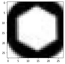
%matplotlib inline
import matplotlib.pyplot as plt
print(y_test[1])
plt.imshow(X_test[1].reshape(28,28), cmap="gray")
plt.show()
np.argmax(pred[1])
87/87 [==============================] - 0s 2ms/step - loss: 0.3534 - accuracy: 0.8467
[1. 0. 0. 0. 0.]
---------------------------------------------------------------------------
NameError                                 Traceback (most recent call last)
~\AppData\Local\Temp/ipykernel_440/1004372224.py in <module>
     11 plt.show()
     12
---> 13 np.argmax(pred[1])

NameError: name 'pred' is not defined
# Kategorien:
# 0: innensechskant
# 1: philips
# 2: pozidriv
# 3: sechskant
# 4: torx

count=0
for i in range(0, len(X_test)):
    # wenn pozidriv vorhergesagt wurde und die richtige Klasse Philips gewesen ist:
    if y_test_pred[i] == 2 and y_test[i] ==1:
        count += 1
        # zeige die Bilder an
        plt.imshow(X_test[i].reshape(28, 28))
        plt.show()
        print(count)
---------------------------------------------------------------------------
ValueError                                Traceback (most recent call last)
~\AppData\Local\Temp/ipykernel_440/1308905088.py in <module>
      9 for i in range(0, len(X_test)):
     10     # wenn pozidriv vorhergesagt wurde und die richtige Klasse Philips gewesen ist:
---> 11     if y_test_pred[i] == 2 and y_test[i] ==1:
     12         count += 1
     13         # zeige die Bilder an

ValueError: The truth value of an array with more than one element is ambiguous. Use a.any() or a.all()
class NeuralNetwork(object):
def __init__(self, lr = 0.1):
self.lr = lr
self.w0 = np.random.randn(100, 784)
self.w1 = np.random.randn(5, 100)
def activation(self, x):
return expit(x)
def train(self, X, y):
a0 = self.activation(self.w0 @ X.T)
pred = self.activation(self.w1 @ a0)
e1 = y.T - pred
e0 = e1.T @ self.w1
dw1 = e1 * pred * (1 - pred) @ a0.T / len(X)
dw0 = e0.T * a0 * (1 - a0) @ X / len(X)
assert dw1.shape == self.w1.shape
assert dw0.shape == self.w0.shape
self.w1 = self.w1 + self.lr * dw1
self.w0 = self.w0 + self.lr * dw0
# print("Kosten: " + str(self.cost(pred, y)))
def predict(self, X):
a0 = self.activation(self.w0 @ X.T)
pred = self.activation(self.w1 @ a0)
return pred
def cost(self, pred, y):
# SUM((y - pred)^2)
s = (1 / 2) * (y.T - pred) ** 2
return np.mean(np.sum(s, axis=0))
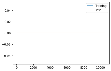
limits = [100, 1000, 3000, 9000, 10500]
test_accs = []
train_accs = []
for limit in limits:
model = NeuralNetwork(0.25)
for i in range(0, 100):
for j in range(0, limit, 100):
model.train(X_train[j:(j + 100), :] / 255., y_train_oh[j:(j + 100), :])
y_test_pred = model.predict(X_test / 255.)
y_test_pred = np.argmax(y_test_pred, axis=0)
test_acc = np.mean(y_test_pred == y_test)
y_train_pred = model.predict(X_train / 255.)
y_train_pred = np.argmax(y_train_pred, axis=0)
train_acc = np.mean(y_train_pred == y_train)
test_accs.append(test_acc)
train_accs.append(train_acc)
plt.plot(limits, train_accs, label="Training")
plt.plot(limits, test_accs, label="Test")
plt.legend()
plt.show()
C:\Users\Martin\anaconda3\envs\py37\lib\site-packages\ipykernel_launcher.py:53: DeprecationWarning: elementwise comparison failed; this will raise an error in the future.
C:\Users\Martin\anaconda3\envs\py37\lib\site-packages\ipykernel_launcher.py:57: DeprecationWarning: elementwise comparison failed; this will raise an error in the future.
C:\Users\Martin\anaconda3\envs\py37\lib\site-packages\ipykernel_launcher.py:19: RuntimeWarning: invalid value encountered in true_divide
C:\Users\Martin\anaconda3\envs\py37\lib\site-packages\ipykernel_launcher.py:20: RuntimeWarning: invalid value encountered in true_divide
class NeuralNetwork(object):
def __init__(self, lr = 0.1):
self.lr = lr
self.w0 = np.random.randn(100, 784)
self.w1 = np.random.randn(5, 100)
def activation(self, x):
return expit(x)
def train(self, X, y):
a0 = self.activation(self.w0 @ X.T)
pred = self.activation(self.w1 @ a0)
e1 = y.T - pred
e0 = e1.T @ self.w1
dw1 = e1 * pred * (1 - pred) @ a0.T / len(X)
dw0 = e0.T * a0 * (1 - a0) @ X / len(X)
assert dw1.shape == self.w1.shape
assert dw0.shape == self.w0.shape
self.w1 = self.w1 + self.lr * dw1
self.w0 = self.w0 + self.lr * dw0
# print("Kosten: " + str(self.cost(pred, y)))
def predict(self, X):
a0 = self.activation(self.w0 @ X.T)
pred = self.activation(self.w1 @ a0)
return pred
def cost(self, pred, y):
# SUM((y - pred)^2)
s = (1 / 2) * (y.T - pred) ** 2
return np.mean(np.sum(s, axis=0))
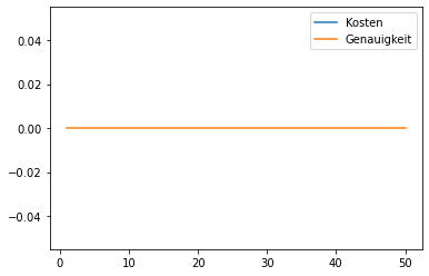
model = NeuralNetwork()
epochs = []
costs = []
accs = []
for i in range(0, 50):
for j in range(0, 10500, 100):
model.train(X_train[j:(j + 100), :] / 255., y_train_oh[j:(j + 100), :])
cost = model.cost(model.predict(X_train), y_train_oh)
y_test_pred = model.predict(X_test / 255.)
y_test_pred = np.argmax(y_test_pred, axis=0)
acc = np.mean(y_test_pred == y_test)
epochs.append(i + 1)
costs.append(cost)
accs.append(acc)
import matplotlib.pyplot as plt
plt.plot(epochs, costs, label="Kosten")
plt.plot(epochs, accs, label="Genauigkeit")
plt.legend()
plt.show()
C:\Users\Martin\anaconda3\envs\py37\lib\site-packages\ipykernel_launcher.py:19: RuntimeWarning: invalid value encountered in true_divide
C:\Users\Martin\anaconda3\envs\py37\lib\site-packages\ipykernel_launcher.py:20: RuntimeWarning: invalid value encountered in true_divide
C:\Users\Martin\anaconda3\envs\py37\lib\site-packages\ipykernel_launcher.py:55: DeprecationWarning: elementwise comparison failed; this will raise an error in the future.
class NeuralNetwork(object):
    def __init__(self, lr = 0.1, hidden_size = 100):
        self.lr = lr

        self.w0 = np.random.randn(hidden_size, 784)
        self.w1 = np.random.randn(5, hidden_size)


    def activation(self, x):
        return expit(x)

    def train(self, X, y):
        a0 = self.activation(self.w0 @ X.T)
        pred = self.activation(self.w1 @ a0)

        e1 = y.T - pred
        e0 = e1.T @ self.w1

        dw1 = e1 * pred * (1 - pred) @ a0.T / len(X)
        dw0 = e0.T * a0 * (1 - a0) @ X / len(X)

        assert dw1.shape == self.w1.shape
        assert dw0.shape == self.w0.shape

        self.w1 = self.w1 + self.lr * dw1
        self.w0 = self.w0 + self.lr * dw0

        # print("Kosten: " + str(self.cost(pred, y)))

    def predict(self, X):
        a0 = self.activation(self.w0 @ X.T)
        pred = self.activation(self.w1 @ a0)
        return pred

    def cost(self, pred, y):
        # SUM((y - pred)^2)
        s = (1 / 2) * (y.T - pred) ** 2
        return np.mean(np.sum(s, axis=0))

for hidden_size in [500, 600, 700, 800]:

    model = NeuralNetwork(0.3, hidden_size)

    for i in range(0, 25):
        for j in range(0, 10500, 100):
            model.train(X_train[j:(j + 100), :] / 255., y_train_oh[j:(j + 100), :])

        # cost = model.cost(model.predict(X_train), y_train_oh)

    y_test_pred = model.predict(X_test / 255.)
    y_test_pred = np.argmax(y_test_pred, axis=0)
    acc = np.mean(y_test_pred == y_test)

    print(str(hidden_size) + ": " + str(acc))
C:\Users\Martin\anaconda3\envs\py37\lib\site-packages\ipykernel_launcher.py:19: RuntimeWarning: invalid value encountered in true_divide
C:\Users\Martin\anaconda3\envs\py37\lib\site-packages\ipykernel_launcher.py:20: RuntimeWarning: invalid value encountered in true_divide
C:\Users\Martin\anaconda3\envs\py37\lib\site-packages\ipykernel_launcher.py:52: DeprecationWarning: elementwise comparison failed; this will raise an error in the future.
500: 0.0
600: 0.0
700: 0.0
800: 0.0